
Graphic Neural Network Model for Screening of Novel Inhibitors for SARS CoV 3C-like Protease
Introduction
This project aims to build a model that would aid novel drug design processes and is hosted here: https://github.com/susanzhang233/mollykill_2.0. Somewhat related to this mollykill 1.0, this project hopes to simplify limitations of the generator and decoder by disregarding GAN’s over-complicated generative structure. In this 2.0 version, we’ll be more focused on employing the accuracy and efficiency of the discriminator. Then, instead of letting the generator to come up with new molecules starting from zero. We’ll be applying a larger real world molecule datasets(ie. Zinc15), to mimic the traditional virtual/actual screening process to come up with potential inhibitors.
Model Structure

Featurizer
To represent the molecules in computer understandable format, this project uses the MolGraphConvFeaturizer from deepchem package that could be referred from here. This featurizer concatenates each molecule’s multiple features into two arrays: nodes array and edges array. Within each of the two arrays, there are then numbers of one-hot encoded arrays corresponding to numbers of atoms in each molecules, i.e. each atom and each bond is represented by one array.
To ensure that the size of the molecule representations are the same(i.e. to standardize input size), this project went one step further to sum up the atom and bond arrays along each column, therefore ending up with node arrays of length 30 and edges array of 11 for each molecule.
Dataset
The example dataset used for demonstration of this model is originally from PubChem AID1706, previously handled by JClinic AIcure team at MIT into this binarized label form. The dataset is also hosted in the data folder of this project.
Repository Explanation
FancyModule.pycontains the major functions of this projectexample.ipynbis an example usage in the model pipeline
Setup
If you are running locally(i.e. in a jupyter notebook in conda, just make sure you installed:
- RDKit
- DeepChem 2.5.0 & above
- Tensorflow 2.4.0 & above
Then, please skip the following part and continue from Data Preparations.
To increase efficiency, we recommend running in Colab.
Then, we’ll first need to run the following lines of code, these will download conda with the deepchem environment in colab.
#!curl -Lo conda_installer.py https://raw.githubusercontent.com/deepchem/deepchem/master/scripts/colab_install.py
#import conda_installer
#conda_installer.install()
#!/root/miniconda/bin/conda info -e
#!pip install --pre deepchem
#import deepchem
#deepchem.__version__
Data Preparations
Now we are ready to import some useful functions/packages, along with our model.
Import Data
import FancyModule##our model
from rdkit import Chem
from rdkit.Chem import AllChem
import pandas as pd
import numpy as np
import matplotlib.pyplot as plt
import deepchem as dc
Select subset for training
Here, for demonstration, we’ll be selecting a subset of size $2405$ from this in-vitro assay that detects inhibition of SARS-CoV 3CL protease via fluorescence.
The dataset is originally from PubChem AID1706, previously handled by JClinic AIcure team at MIT into this binarized label form.
df = pd.read_csv('AID1706_binarized_sars.csv')
df_false = df[df['activity']==0].sample(n=2000, replace = False)#s
df_true = df[df['activity'] == 1]
df_subset = pd.concat([df_false, df_true], ignore_index = True)
df_subset
| smiles | activity | |
|---|---|---|
| 0 | C1=CC=C(C(=C1)C(=O)O)N=NC2=C(NC3=C2C=C(C=C3)[N... | 0 |
| 1 | COC1=CC=CC=C1C2=NN(C(=O)C=C2)CC(=O)NC3CCC4=CC=... | 0 |
| 2 | CN(C)C(=S)NC1=CC=C(C=C1)CC2=CC=NC=C2 | 0 |
| 3 | CC1=CC(=NC2=CC=CC=C12)SCC(=O)C3=C(N(C(=C3)C)C)C | 0 |
| 4 | CN(CC1=CC(=NN1)COC)C(=O)C2CCC(=O)N(C2)CC3=CC(=... | 0 |
| ... | ... | ... |
| 2400 | C1COC2=C(O1)C=CC(=C2)NC(=O)C3=C(OC=N3)C4=CC=CC=C4 | 1 |
| 2401 | COC(=O)C1=CC=CC=C1NC(=O)C2=CC3=C(C=C2)OCCCO3 | 1 |
| 2402 | COC1=CC=CC=C1CCNC(=O)C(=O)NCC2N(CCO2)S(=O)(=O)... | 1 |
| 2403 | CN(C)CCNC(=O)C(=O)NCC1N(CCO1)S(=O)(=O)C2=CC=C(... | 1 |
| 2404 | C1COC(N1S(=O)(=O)C2=CC3=C(C=C2)OCCO3)CNC(=O)C(... | 1 |
2405 rows × 2 columns
Observe the dataframe above, it contains a ‘smiles’ column, which stands for the smiles representation of the molecules. There is also an ‘activity’ column, in which it is the label specifying whether that molecule is considered as hit for the protein.
Set Minimum Length for molecules
Since we’ll be using graphic representation for each molecules, we’ll first need to cast the molecules into one universal length to fit into our training model. Our module contains a preparation function prepare_data that eliminates molecules shorter than the desired size.
df_minlength, y = FancyModule.prepare_data(df_subset, 12)
Featurization
Our module also have a featurize function that represents the molecules in graphic format that is supported by our model. The main structure of the featurizer could be referred from here.
Note: the original featurizer was modified for usage in this project.
Supported with input_df, the function would return featurized node and edges.
nodes, edges = FancyModule.featurize(df_minlength['smiles'])
Training
Now, we’re finally ready for training. We’ll first import some necessary functions from tensorflow.
import tensorflow as tf
from tensorflow import keras
from tensorflow.keras import layers
Here we’ll first initiate a model with the corresponding make_model functions in the package.
model = FancyModule.make_model()
Now we’ll train the model with the above subset and plot out the training curve.
model.compile(optimizer='adam',
              loss=tf.keras.losses.BinaryCrossentropy(from_logits=True),
              metrics=['accuracy'])

history = model.fit([np.array(nodes), np.array(edges)],
                    y,
                    epochs=80,
                    verbose = False,
                    #class_weight=class_weights
                    #steps_per_epoch = 100,
                    )
plt.plot(history.history["accuracy"])
plt.gca().set(xlabel = "epoch", ylabel = "training accuracy")
[Text(0.5, 0, 'epoch'), Text(0, 0.5, 'training accuracy')]
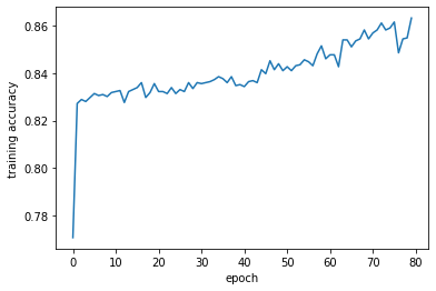
Observe the training curve, the accuracy has a steady growing trend, and the model ultimately achieved an accuracy of around 86 percent.
Testing (Payoff)
Finally, we’ll demonstrate the testing phase(thoroughput screening) with a newly random selected subset from the above mentioned SARS-CoV 3CL protease assay.
df_false = df[df['activity']==0].sample(n=2000, replace = False)#s

df_test_subset = pd.concat([df_false, df_true], ignore_index = True)
The testing function accepts three parameters: the testing column of molecules in smiles format, trained model, and True/False statement of whether to save the result in the directory(default False).
FancyModule.test(df_test_subset['smiles'], model)
| smiles | prediction | |
|---|---|---|
| 1756 | C([C@@H]1[C@H]([C@@H]([C@H]([C@H](O1)O[C@H]([C... | 0.999190 |
| 2055 | C1=CC=C2C(=C1)C(=CC(=C2N)C(C(F)(F)F)(C(F)(F)F)... | 0.998951 |
| 2093 | C1=CC(=CC(=C1)NC(=O)NCCNC(=O)C2=C(C=CC(=C2)OCC... | 0.995320 |
| 2234 | C1=CC(=CC=C1/C(=N/S(=O)(=O)C2=CC(=CC(=C2)C(F)(... | 0.993566 |
| 1713 | CC(C)CC(COCC1=CC=C(C=C1)C(F)(F)F)N2CCN(CCC2=O)... | 0.991890 |
| ... | ... | ... |
| 202 | CC1CC2C3CCC4CC(CCC4(C3=CCC2(C1(C(=O)C)O)C)C)O | 0.000008 |
| 125 | CC#CC[N+](C)(CC#CC)CC(=O)C1=CC=CC=C1.[Br-] | 0.000004 |
| 501 | CCOC(=O)N1CCN(CC1)C(=O)C2CCC(CC2)C(=O)N3CCN(CC... | 0.000003 |
| 540 | CC(=O)OC1C2CCC1C(CC2)[N+]3(CCCCC3)C.[I-] | 0.000002 |
| 454 | CC1(CC(CC(N1)(C)C)N2CN(CC2=O)C3CCCCC3)C | 0.000002 |
2405 rows × 2 columns
Yay, now we have our output data table. It has two columns, smiles format of molecules, and their corresponding prediction of inhibition score to the protein target, as estimated by our model.
Limitations(Future work)
- Currently, the model accuracy is around 86-88%. More attempts with different model structure might be tested for possible improvements.
- The efficiency of the featurization and training process might be improved.
- Future wet-lab experiments could be done for confirmation from another aspect.
Acknowledgements
- Featurizer https://deepchem.readthedocs.io/en/latest/api_reference/featurizers.html#deepchem.feat.MolGraphConvFeaturizer
- Featurizer paper https://arxiv.org/pdf/1603.00856.pdf