
Blog Post 3 - Fake News Classifier
In this blog, we’ll build a machine learning model with Tensorflow that helps us to classify fake news.
First, we’ll import some of the needed packages our dataset to feed the model.
import pandas as pd
import tensorflow as tf
import numpy as np
from matplotlib import pyplot as plt
Both the training and testing datasets are accessed from Kaggle:
#train_url = "https://github.com/PhilChodrow/PIC16b/blob/master/datasets/fake_news_train.csv?raw=true"
df = pd.read_csv('fake_news_train.csv')
test_url = "https://github.com/PhilChodrow/PIC16b/blob/master/datasets/fake_news_test.csv?raw=true"
test_df = pd.read_csv(test_url)
df
| Unnamed: 0 | title | text | fake | |
|---|---|---|---|---|
| 0 | 17366 | Merkel: Strong result for Austria's FPO 'big c... | German Chancellor Angela Merkel said on Monday... | 0 |
| 1 | 5634 | Trump says Pence will lead voter fraud panel | WEST PALM BEACH, Fla.President Donald Trump sa... | 0 |
| 2 | 17487 | JUST IN: SUSPECTED LEAKER and “Close Confidant... | On December 5, 2017, Circa s Sara Carter warne... | 1 |
| 3 | 12217 | Thyssenkrupp has offered help to Argentina ove... | Germany s Thyssenkrupp, has offered assistance... | 0 |
| 4 | 5535 | Trump say appeals court decision on travel ban... | President Donald Trump on Thursday called the ... | 0 |
| ... | ... | ... | ... | ... |
| 22444 | 10709 | ALARMING: NSA Refuses to Release Clinton-Lynch... | If Clinton and Lynch just talked about grandki... | 1 |
| 22445 | 8731 | Can Pence's vow not to sling mud survive a Tru... | () - In 1990, during a close and bitter congre... | 0 |
| 22446 | 4733 | Watch Trump Campaign Try To Spin Their Way Ou... | A new ad by the Hillary Clinton SuperPac Prior... | 1 |
| 22447 | 3993 | Trump celebrates first 100 days as president, ... | HARRISBURG, Pa.U.S. President Donald Trump hit... | 0 |
| 22448 | 12896 | TRUMP SUPPORTERS REACT TO DEBATE: “Clinton New... | MELBOURNE, FL is a town with a population of 7... | 1 |
22449 rows × 4 columns
Apart from the indices column, the dataframe contains three more informative columns: title column, the titles of the news; text column, the content of that news; the fake column, label indicating whether the news is 0(real), or 1(fake).
Make Dataset
Before we actually start the training process, transforming the dataset into decent forms for training are also very important. Here, we’ll create a make_dataset function that’ll do two things:
-
remove stop words from the article text and title columns(stop words refers to those most common words in a language, which could be filtered out for training. Some common stop words are a, the, as, at, by, to, etc)
-
construct a tensorflow dataset with inputs (title, text) and output fake column labels. Dataset format of enables the input to be smoothly handled by tensorflow (tensorflow dataset is a specific class containing many useful functions to keep you organized)
To remove stop words, we’ll first import some extra packages and functions.
- the
stop wordsfunction gives you a list of common stop words of specified language; - the
word_tokenizefunction breaks a string into single words and punctuations of a 1d array form; - the
TreebankWordDetokenizerfunction detokenizes a 1d array of words, combining it back into one individual string.
import nltk
#nltk.download('stopwords') #only need to be downloaded once
#nltk.download('punkt')  #only need to be downloaded once as well
from nltk.corpus import stopwords
from nltk.tokenize import word_tokenize
stop = stopwords.words('english')
from nltk.tokenize.treebank import TreebankWordDetokenizer
def make_dataset(df):
    df_ = df

    #remove stopwords for the dataframe
    df_['title'] = df_['title'].apply(word_tokenize)# split a string into separate tokens
    df_['title'] = df['title'].apply(lambda x: [w for w in x if not w in stop] )#remove stopwords
    df_['text'] = df_['text'].apply(word_tokenize)
    df_['text'] = df_['text'].apply(lambda x: [w for w in x if not w in stop] )
    df_['text'] = df_['text'].apply(lambda x: TreebankWordDetokenizer().detokenize(x))#combine the tokens back to a complete sentence
    df_['title'] = df_['title'].apply(lambda x: TreebankWordDetokenizer().detokenize(x))

    #create tensorflow dataset with inputs (title, text) and output fake column labels and return it
    return tf.data.Dataset.from_tensor_slices(({"title": df_['title'], "text": df_['text']}, df_['fake']))
We then apply the function to our training and testing datasets:
dataset = make_dataset(df)
test_dataset = make_dataset(test_df)
Train Validation Split, Create Batches
Now we are ready to construct some train & validation split inside our training set. Along with that, we’ll also set batches for training set, as training with the original dataset volume might be too inefficient for demonstration purposes.
#shuffle the complete training set
dataset = dataset.shuffle(buffer_size = len(dataset))

#specify training and validation size: 0.7 & 0.2, respectively
train_size = int(0.7*len(dataset))
val_size   = int(0.2*len(dataset))

#pick out first 0.7 as training set, with a batch of 100
train = dataset.take(train_size).batch(100)
#pick out the next 0.2 as validation set, with a batch of 100
val   = dataset.skip(train_size).take(val_size).batch(100)
#test  = dataset.skip(train_size + val_size).batch(100) #last 0.1 of data

#check for the length of the two sets
len(train), len(val)#, len(test)
(158, 45)
test_ds = test_dataset.batch(100)
Create Models
We are now ready to make our models. While our data contains informative columns of both news title and news text, we would like to know whether titles only, text only, or both, would be more effective for detection of fake news. Therefore, we’ll be creating three models, with similar strategies, and comparing their accuracies.
Vectorization layer
No matter which combination we’ll be using, we all need to first vectorize the input strings. Vectorization refers to processing of the strings into computer readable format, which is, numbers. There are multiple ways of vectorization of strings, such as the term-document matrix, etc. Here, we’ll be using the TextVectorization function provided by tensorflow. This function would represent each of the words by its rank of frequency in the whole dataset. First, we’ll need to define a standardization function to supply to the TextVectorization function.
Here, the standardization function would convert all words to lowercases and remove all punctuations.
def standardization(input_data):
    lowercase = tf.strings.lower(input_data)
    no_punctuation = tf.strings.regex_replace(lowercase,
                                  '[%s]' % re.escape(string.punctuation),'')
    return no_punctuation
Then, with the TextVectorization function, we’ll make a vectorize_layer that transforms each words in the training set, after standardization treatment, into tensors with the words’ corresponding frequency rank.
from tensorflow.keras import losses
from tensorflow.keras.layers.experimental.preprocessing import TextVectorization

import re
import string
# only the first 2000 distinct words in the whole set will be tracked
max_tokens = 2000

# only the first 20 words of each headline will be considered
sequence_length = 20

vectorize_layer = TextVectorization(
    standardize=standardization,
    max_tokens=max_tokens, # only consider this many words
    output_mode='int',
    output_sequence_length=sequence_length)
After creating the layers, we would still need to adapt the layer to our set. By adapting it, we will ensure that the vectorization layer have the words’ corresponding frequency ranks fixed. Thus whenever we are training or testing with that layer, each distinct word would have that one and only ranking.
vectorize_layer.adapt(train.map(lambda x, y: x["title"]))
vectorize_layer.adapt(train.map(lambda x, y: x["text"]))
Then, we’ll specify two input layers for title and text.
from tensorflow import keras
from tensorflow.keras import layers
title_input = keras.Input(
    shape = (1,),
    name = "title",
    dtype = "string"
)

text_input = keras.Input(
    shape = (1,),
    name = "text",
    dtype = "string"
)
Model trains with titles only
Since we have two kinds of inputs, title and text, we’ll be using the keras functional API, instead of sequential API. The functional API can create layers that have more flexible sequences, therefore suitable for building a model with multiple inputs. First, we’ll build a model that learns the news titles only.
Our first layer would be the vectorize_layer we just built. In each of the following layers, we supply the input as the result obtained from the preceding layer in ().
With Dropout, the input units in that layer will be set to 0 with a frequency of rate at each step during training time, which helps prevent overfitting.
The Embedding layer creates a vocabulary space, giving each word its own unique spot in that space. Furthermore, the spots of the words are set in a way that the distance and direction between words would indicate relatedness and relationships. We’ll give this layer a name “embedding_tl” to ease the process of examining it later.
x = vectorize_layer(title_input)
x = layers.Embedding(max_tokens, output_dim = 5, name = "embedding_tl")(x)
x = layers.Dropout(0.2)(x)
x = layers.GlobalAveragePooling1D()(x)
x = layers.Dropout(0.2)(x)
x = layers.Dense(32, activation='relu')(x)
output = layers.Dense(2, name = "fake")(x)
Now, we are finally ready to build the model. Only specifying the initial input, tensorflow will be able to extract all that information we’ve provided of the layers.
model_tl = keras.Model(
    inputs = title_input,
    outputs = output
)
model_tl.summary()
Model: "model"
_________________________________________________________________
Layer (type)                 Output Shape              Param #
=================================================================
title (InputLayer)           [(None, 1)]               0
_________________________________________________________________
text_vectorization (TextVect (None, 20)                0
_________________________________________________________________
embedding_tl (Embedding)     (None, 20, 5)             10000
_________________________________________________________________
dropout (Dropout)            (None, 20, 5)             0
_________________________________________________________________
global_average_pooling1d (Gl (None, 5)                 0
_________________________________________________________________
dropout_1 (Dropout)          (None, 5)                 0
_________________________________________________________________
dense (Dense)                (None, 32)                192
_________________________________________________________________
fake (Dense)                 (None, 2)                 66
=================================================================
Total params: 10,258
Trainable params: 10,258
Non-trainable params: 0
_________________________________________________________________
As always, we’ll compile the model and fit it to the training set.
model_tl.compile(optimizer = "adam",
              loss = losses.SparseCategoricalCrossentropy(from_logits=True),
              metrics=['accuracy']
)
history = model_tl.fit(train,
                    validation_data=val,
                    epochs = 50,
                    verbose = False)
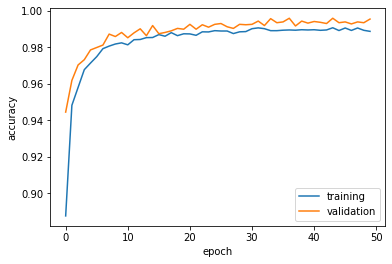
And we’ll plot out the accuracy curve.
plt.plot(history.history["accuracy"], label = "training")
plt.plot(history.history["val_accuracy"], label = "validation")
plt.gca().set(xlabel = "epoch", ylabel = "accuracy")
plt.legend()
model_tl.evaluate(test_ds)
225/225 [==============================] - 0s 1ms/step - loss: 0.0840 - accuracy: 0.9752


[0.08402662724256516, 0.9751881957054138]
Evaluating the model with only titles with out test set, we could see that the accuracy is actually pretty high: 0.97! Let’s see if the other two models could do better.S
Model trains with text only
Training with text would have a similar process: specify each layers, make the model, compile it, fit it, evaluate and observe.
x_ = vectorize_layer(text_input)
x_ = layers.Embedding(max_tokens, output_dim = 5, name = "embedding_tx")(x_)
x_ = layers.Dropout(0.2)(x_)
x_ = layers.GlobalAveragePooling1D()(x_)
x_ = layers.Dropout(0.2)(x_)
x_ = layers.Dense(32, activation='relu')(x_)
output = layers.Dense(2, name = "fake")(x_)
model_tx= keras.Model(
    inputs = text_input,
    outputs = output
)
model_tx.compile(optimizer = "adam",
              loss = losses.SparseCategoricalCrossentropy(from_logits=True),
              metrics=['accuracy']
)
model_tx.fit(train,
                    validation_data=val,
                    epochs = 50,
                    verbose = False)
model_tx.evaluate(test_ds)
225/225 [==============================] - 1s 6ms/step - loss: 0.1612 - accuracy: 0.9463


[0.16124901175498962, 0.9462782144546509]
The accuracy for the model trained with the text only has a lower accuracy. Somehow reasonable, as the text is longer, and a fake news might also possess some sentences that sounds true.
Model trained with both text and title
both = layers.concatenate([x, x_], axis = 1)
output_both = layers.Dense(2, name = "fake")(both)
model_both= keras.Model(
    inputs = [title_input, text_input],
    outputs = output_both
)
model_both.summary()
Model: "model_2"
__________________________________________________________________________________________________
Layer (type)                    Output Shape         Param #     Connected to
==================================================================================================
title (InputLayer)              [(None, 1)]          0
__________________________________________________________________________________________________
text (InputLayer)               [(None, 1)]          0
__________________________________________________________________________________________________
text_vectorization (TextVectori (None, 20)           0           title[0][0]
                                                                 text[0][0]
__________________________________________________________________________________________________
embedding_tl (Embedding)        (None, 20, 5)        10000       text_vectorization[0][0]
__________________________________________________________________________________________________
embedding_tx (Embedding)        (None, 20, 5)        10000       text_vectorization[1][0]
__________________________________________________________________________________________________
dropout (Dropout)               (None, 20, 5)        0           embedding_tl[0][0]
__________________________________________________________________________________________________
dropout_2 (Dropout)             (None, 20, 5)        0           embedding_tx[0][0]
__________________________________________________________________________________________________
global_average_pooling1d (Globa (None, 5)            0           dropout[0][0]
__________________________________________________________________________________________________
global_average_pooling1d_1 (Glo (None, 5)            0           dropout_2[0][0]
__________________________________________________________________________________________________
dropout_1 (Dropout)             (None, 5)            0           global_average_pooling1d[0][0]
__________________________________________________________________________________________________
dropout_3 (Dropout)             (None, 5)            0           global_average_pooling1d_1[0][0]
__________________________________________________________________________________________________
dense (Dense)                   (None, 32)           192         dropout_1[0][0]
__________________________________________________________________________________________________
dense_1 (Dense)                 (None, 32)           192         dropout_3[0][0]
__________________________________________________________________________________________________
concatenate (Concatenate)       (None, 64)           0           dense[0][0]
                                                                 dense_1[0][0]
__________________________________________________________________________________________________
fake (Dense)                    (None, 2)            130         concatenate[0][0]
==================================================================================================
Total params: 20,514
Trainable params: 20,514
Non-trainable params: 0
__________________________________________________________________________________________________
model_both.compile(optimizer = "adam",
              loss = losses.SparseCategoricalCrossentropy(from_logits=True),
              metrics=['accuracy']
)
model_both.fit(train,
                    validation_data=val,
                    epochs = 50,
                    verbose = False)
<tensorflow.python.keras.callbacks.History at 0x7f84c388e910>
model_both.evaluate(test_ds)
225/225 [==============================] - 1s 6ms/step - loss: 0.0371 - accuracy: 0.9913


[0.037129346281290054, 0.991313636302948]
Here, we could observe that training with both text and title yields an accuracy of 0.9913!
Embedding Analysis
In the next stage, we’ll extract the previous Embedding layer, do some visualization of it to demonstrate how the words are learned by the model. We’ll plot out each word’s spot in the whole 2d vocabulary space. Since our embedding layer has an output of 5 dimensions, we’ll first need to conduct principle component analysis to transform it into 2d representations. Sci-kit learn has that function created for us.
First, we’ll get the vocabularies and weights corresponding to the words in the two embedding layers of title/text out:
weights_tl = model_both.get_layer('embedding_tl').get_weights()[0]
weights_tx = model_both.get_layer('embedding_tx').get_weights()[0]# get the weights from the embedding layer
vocab = vectorize_layer.get_vocabulary()
vocab = vectorize_layer.get_vocabulary()
weights_tl
array([[ 0.10268341,  0.09916885, -0.11284392,  0.12111397, -0.10344727],
       [-0.10890676, -0.13384679,  0.10487777, -0.12676527,  0.13442   ],
       [ 0.05327572,  0.05760193, -0.11840718, -0.00806848, -0.11700375],
       ...,
       [ 0.02861674,  0.02574723,  0.04686182,  0.09227268, -0.03490727],
       [ 0.15639482,  0.09743544, -0.06591856,  0.02370312, -0.01798774],
       [ 0.00066107, -0.01369754, -0.06120993,  0.03191474, -0.09007049]],
      dtype=float32)
Next, we perform PCA to the weights to convert them into 2d arrays:
from sklearn.decomposition import PCA
pca = PCA(n_components=2)
weights_tl = pca.fit_transform(weights_tl)
weights_tx = pca.fit_transform(weights_tx)
len(vocab)
2000
Then, we’ll create a data frame containing the embedding of words in titles.
embedding_tl = pd.DataFrame({
    'word' : vocab,
    'x0'   : weights_tl[:,0],
    'x1'   : weights_tl[:,1]
})
embedding_tl
| word | x0 | x1 | |
|---|---|---|---|
| 0 | -0.195497 | 0.003443 | |
| 1 | [UNK] | 0.317627 | 0.025609 |
| 2 | said | -0.105505 | -0.010339 |
| 3 | trump | 0.100054 | -0.045148 |
| 4 | the | 1.743519 | -0.003649 |
| ... | ... | ... | ... |
| 1995 | tonight | 0.910266 | 0.059968 |
| 1996 | repeated | 0.170522 | 0.024102 |
| 1997 | projects | -0.014011 | -0.052086 |
| 1998 | outcome | -0.117215 | 0.046006 |
| 1999 | launch | -0.029681 | -0.028275 |
2000 rows × 3 columns
We’ll do the same thing with the embedding of words in the news text.
embedding_tx = pd.DataFrame({
    'word' : vocab,
    'x0'   : weights_tx[:,0],
    'x1'   : weights_tx[:,1]
})
Now, we are finally ready to plot the words and their embeddings out!We’ll be using plotly express function!
import plotly.express as px
import plotly.io as pio
pio.templates.default = "plotly_white"
import plotly.express as px
fig = px.scatter( embedding_tl,
                 x = "x0",
                 y = "x1",
                 size = list(np.ones(len(embedding_tl))),
                 size_max = 2,
                 hover_name = "word")

fig.show()
Here, the graph demonstrates each words’ spot in the vocabulary space.
from plotly.io import write_html
write_html(fig, "emb_tx.html")