In this blog post, I’ll write a tutorial on a simple version of the spectral clustering algorithm for clustering data points.

Introduction

Spectral clustering is an important tool for identifying meaningful parts of data sets with complex structure. According to wikipedia, “spectral clustering techniques make use of the spectrum (eigenvalues) of the similarity matrix of the data to perform dimensionality reduction before clustering in fewer dimensions”.

In this blog, we’ll build similarity matrix, generate labels(spectrum) for points, incorporate eigenvalues for creating labels, and ultimately plot out data points into clusters that resemble the pattern on Gary’s shell.

To start, we’ll look at some examples where kmeans are enough for clustering and we don’t need spectral clustering.

Notation

In all the math below:

• Boldface capital letters like \(\mathbf{A}\) refer to matrices (2d arrays of numbers).
• Boldface lowercase letters like \(\mathbf{v}\) refer to vectors (1d arrays of numbers).
• \(\mathbf{A}\mathbf{B}\) refers to a matrix-matrix product (A@B). \(\mathbf{A}\mathbf{v}\) refers to a matrix-vector product (A@v).

import numpy as np
from sklearn import datasets
from matplotlib import pyplot as plt

n = 200
np.random.seed(1111)
X, y = datasets.make_blobs(n_samples=n, shuffle=True, random_state=None, centers = 2, cluster_std = 2.0)
plt.scatter(X[:,0], X[:,1])

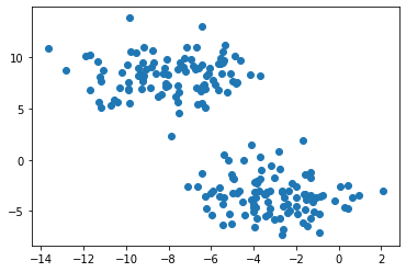
make_blobs function from sklearn would generate to random natural blobs. The output matrix X contains coordinates of the data points, while y contains the labels of each point. K-means is a very common way to achieve clustering task, which has good performance on circular-ish blobs like these:

from sklearn.cluster import KMeans
km = KMeans(n_clusters = 2)
km.fit(X)

plt.scatter(X[:,0], X[:,1], c = km.predict(X))

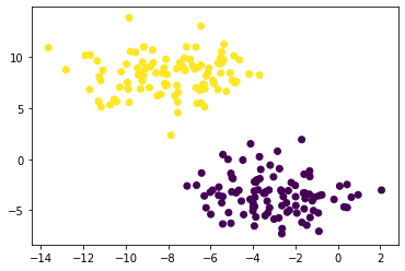
It seems like the kmeans function performs well on blob like datasets. However, what if the datasets have clusters that are apparent by human eye, but could not be clustered out by kmeans?

Harder Clustering

np.random.seed(1234)
n = 200
X, y = datasets.make_moons(n_samples=n, shuffle=True, noise=0.05, random_state=None)
plt.scatter(X[:,0], X[:,1])

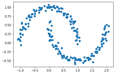
The make_moons function would make out two crescent shape datasets. K-means won’t work so well here, because k-means is designated to optimize clusters with the nearest mean, therefore it would look for circular clusters.

km = KMeans(n_clusters = 2)
km.fit(X)
plt.scatter(X[:,0], X[:,1], c = km.predict(X))

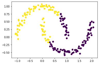
It seems that kmeans won’t work well with crescents.

As we’ll see, spectral clustering are nice in clustering data points that could not be separated by locating centers and spreads.

Part A: Similarity matrix

The first step of spectral clustering would involve constructing the similarity matrix \(\mathbf{A}\). Similarity matrix should be of shape (n, n), with n being the number of total data points. Specifically, the similarity matrix contains information about whether the distance between each pair of the data points is under the specified epsilon threshold.

Entry A[i,j] should be equal to 1 if the distance between the ith and jth data points is within distance epsilon, and would be equal to 0 if otherwise.

The diagonal entries A[i,i] of the matrix is intentionally made to be all be equal to zero.

To calculate the distance between each pair of data points(with their coordinates), we’ll be using the pairwise_distances function from scikit learn. This function does the exact job as mentioned above: given a matrix with n data points with coordinates, the function outputs an n*n matrix containing the distance calculated from the coordinates for each pair of data points.

from sklearn.metrics.pairwise import pairwise_distances

A = pairwise_distances(X)

Then, with the generated pairwise distance matrix, we’ll check if each of the values is within the specified epsilon threshold. If the pairwise distance matrix’s [i,j] entry is within the threshold, then this indicates that the ith data point and the jth data point is close enough to be considered into one cluster, this closeness would thus be represented by a 1 in the similarity matrix \(\mathbf{A}\). Vice versa for points that are not so close, and the far-awayness would be represented by a 0 in the similarity matrix \(\mathbf{A}\).

For this part, we’ll use an epsilon of 0.4.

epsilon = 0.4

A = np.where(A<=epsilon, 1.0, 0.0) #set close pairs of i,js as 1s in the similarity matrix, 0 otherwise
np.fill_diagonal(A , 0)

#draft version:
#epsilon = 0.4
#A[A<=epsilon] = 1 
#A[A !=1 ] = 0 #vice versa
#the diagonal line of A should all be zeros

A

array([[0., 0., 0., ..., 0., 0., 0.],
       [0., 0., 0., ..., 0., 0., 0.],
       [0., 0., 0., ..., 0., 1., 0.],
       ...,
       [0., 0., 0., ..., 0., 1., 1.],
       [0., 0., 1., ..., 1., 0., 1.],
       [0., 0., 0., ..., 1., 1., 0.]])

Now, our similarity matrix is expected to indicate whether the each pair of points in the dataset is close to each other.

Part B: Binary Norm Cut Objective

Now, we have the similarity matrix ready, but we still need some extra tasks to cluster the points into groups.

Let \(C_0\) and \(C_1\) be two clusters of the data points. We’ll define the binary norm cut objective of a matrix \(\mathbf{A}\) for the two clusters, which is the function:

The normalized cut criterion measures both the total dissimilarity between the different groups as well as the total similarity within the groups. The similarity is measured as the distance between data points. Thus combining the inter-group dissimilarity and the intra-group similarity as a binary norm cut term gives a new objective way for clustering.

From the similarity matrix obtained above, let \(d_i = \sum_{j = 1}^n a_{ij}\) be the \(i\)th row-sum of \(\mathbf{A}\), which is also called the degree of \(i\). The degree of \(i\) is thus how many data points, from our similarity matrix, is believed to be in the same cluster as the \(i\)th data point. \(C_0\) and \(C_1\) is still the two only possible clusters of the data points. y contains information of the cluster label for the data points: if y[i] = 1, then point i (and therefore row \(i\) of \(\mathbf{A}\)) is an element of cluster \(C_1\), vice versa.

In the binary norm cut objective function,

• \(\mathbf{cut}(C_0, C_1) \equiv \sum_{i \in C_0, j \in C_1} a_{ij}\) is the cut of the clusters \(C_0\) and \(C_1\): the cut term is the number of entries in \(\mathbf{A}\) that relate points in cluster \(C_0\) to points in cluster \(C_1\). The smaller the value, the more dissimilar the two groups.

• \(\mathbf{vol}(C_0) \equiv \sum_{i \in C_0}d_i\), where \(d_i = \sum_{j = 1}^n a_{ij}\) is the degree of row \(i\) (the total number of all other rows related to row \(i\) through \(A\)). The volume of clusters measure the size of them.

A pair of clusters \(C_0\) and \(C_1\) is considered to be a “good” partition of the data when \(N_{\mathbf{A}}(C_0, C_1)\) is small, as it indicates that there is decent dissimilarity between the two groups, and neither group has significantly small size.

Now, let’s look at how to calculate each of the two factors in this objective function separately.

B.1 The Cut Term

First, as mentioned above, the cut term \(\mathbf{cut}(C_0, C_1)\) is the number of nonzero entries in \(\mathbf{A}\) that relate points in cluster \(C_0\) to points in cluster \(C_1\). In general, the smaller the value, the more dissimilar the two groups.

Here, the cut(A,y) function would compute the cut term. It would sum up the entries A[i,j] for each pair of points (i,j) that are indicated to be in different clusters from the y label container. We could simply sum up the entries to obtain the cut term because the similarity matrix A only contains 0 or 1, with 1 indicating the corresponding i and j data points are close enough to be considered related.

def cut(A,y):
    
    cut = 0

    for i in range(len(y)):
        for j in range(len(y)):
            if y[i] != y[j]: # if y array indicate that i & j shouldn't be in one cluster
                cut += A[i,j] 
                #print('yeah')
    return cut
            

Now, we’ll compare the cut objective we’ve calculated for the true clusters y with some random labels we’ll generate of the same length n. It is expected that the cut objective for the true labels is much smaller than the cut objective for the random labels, since the true clusters is expected to be internally more closely related than the random ones.

randv = np.random.randint(0, 2, size = (n))
cut(A,y), cut(A,randv)

(26.0, 2232.0)

A cut objective of 26 for the true cluster is indeed small enough to be considered legit.

B.2 The Volume Term

Now take a look at the second factor in the norm cut objective. This is the volume term. As mentioned above, the volume of clusters measure how “big” they are. If we choose cluster \(C_0\) to be small, then \(\mathbf{vol}(C_0)\) will be small and \(\frac{1}{\mathbf{vol}(C_0)}\) will be large, leading to an undesirable higher objective value.

Mathematically, \(\mathbf{vol}(C_0) \equiv \sum_{i \in C_0}d_i\), where \(d_i = \sum_{j = 1}^n a_{ij}\) is the degree of row \(i\) (the total number of all other rows related to row \(i\) through \(A\)). Then the volume for the two clusters are thus the sum of the degrees for each row in that cluster.

For the vols(A,y) function, it computes the volumes of \(C_0\) and \(C_1\), returning them as a tuple. A is the similiarity matrix to be calculated, and y is the label for each row(or column). For example, v0, v1 = vols(A,y) should result in v0 holding the volume of cluster 0 and v1 holding the volume of cluster 1.

def vols(A, y):
    
    v1 = A[y==1].sum() #degree sum for rows corresponding points in C1
    
    v0 = A[y==0].sum() #that of C0
    
    return v0,v1

Then, we’ll ultimately develop the normcut(A,y) function. This function is expected to integrate cut(A,y) and vols(A,y) to compute the binary normalized cut objective of a matrix A with clustering vector y.

def normcut(A,y):
    v0,v1 = vols(A,y)
    return cut(A,y) * (1/v0 + 1/v1)

As mentioned above, for two ‘good’ clusters, the binary normcut objective is expected to be small enough so that:

• it minimizes number of entries in the similarity matrix A that indicates relatedness for points in different clusters: small cut term
• neither clusters should be too small: small volume term

Now, we’ll use the normcut function to check that the normcut objective of the true labels y is indeed small, at least smaller than that from generated random fake labels.

normcut(A,y), normcut(A,randv)

(0.02303682466323045, 1.991672673470162)

The normcut for the true labels are indeed smaller than that from the fake labels! This demonstrates that the true clusters are ideal clusters that meets the bi-normcut criterions above.

Part C: \(z\) vector as representation for vol terms

The above part demonstrated the binary normcut criterion for clustering tasks. In other words, the process of clustering is actually a process of looking for y labels that minimizes the normcut objective value. However, this minimization process might require too much computational work with calculating the actual vol term. In fact, there is a way to make the vol term calculation more efficient.

Here’s a mathematic trick:

we’ll define a new vector \(\mathbf{z} \in \mathbb{R}^n\) such that:

In the above function, \(y_i\) is the cluster identity of point i, therefore, if \(i\) is in cluster \(C_0\), \(z_i > 0\) and vice versa. Instead of having multiple values that are hard to comprehend, this \(z\) vector contains all the informations needed in signs: positive z and negative z corresponding to the two clusters.

Now, we create a transform function that takes in A and y, returning a corresponding \(z\) vector that contains the volume term informations, with clusters indicated by signs, as mentioned above.

def transform(A , y):
    v0,v1 = vols(A,y)
    z = np.where(y==1,  -1/v1 , 1/v0 )
    return z

#D = np.ndarray((n,n) )
#np.fill_diagonal(D, np.sum(A,axis=1) )
D = np.diag(np.sum(A,axis=1))
z = transform(A , y)

Take a look at the \(z\) vector we’ve obtained. Yup, it indeed is a vector with only two unique values of different signs.

z

array([-0.00045106, -0.00045106,  0.00043497,  0.00043497,  0.00043497,
        0.00043497,  0.00043497,  0.00043497, -0.00045106, -0.00045106,
       -0.00045106,  0.00043497, -0.00045106, -0.00045106, -0.00045106,
       -0.00045106, -0.00045106,  0.00043497,  0.00043497,  0.00043497,
       -0.00045106, -0.00045106, -0.00045106,  0.00043497,  0.00043497,
       -0.00045106,  0.00043497, -0.00045106, -0.00045106,  0.00043497,
        0.00043497, -0.00045106, -0.00045106, -0.00045106, -0.00045106,
       -0.00045106,  0.00043497, -0.00045106, -0.00045106,  0.00043497,
       -0.00045106,  0.00043497,  0.00043497,  0.00043497,  0.00043497,
        0.00043497,  0.00043497, -0.00045106, -0.00045106, -0.00045106,
        0.00043497,  0.00043497, -0.00045106, -0.00045106,  0.00043497,
        0.00043497, -0.00045106, -0.00045106, -0.00045106,  0.00043497,
        0.00043497,  0.00043497, -0.00045106,  0.00043497, -0.00045106,
        0.00043497,  0.00043497,  0.00043497,  0.00043497, -0.00045106,
       -0.00045106, -0.00045106, -0.00045106,  0.00043497,  0.00043497,
        0.00043497, -0.00045106,  0.00043497, -0.00045106,  0.00043497,
        0.00043497,  0.00043497,  0.00043497, -0.00045106, -0.00045106,
       -0.00045106, -0.00045106,  0.00043497,  0.00043497,  0.00043497,
        0.00043497, -0.00045106,  0.00043497,  0.00043497, -0.00045106,
       -0.00045106, -0.00045106, -0.00045106,  0.00043497,  0.00043497,
       -0.00045106, -0.00045106, -0.00045106,  0.00043497, -0.00045106,
       -0.00045106,  0.00043497,  0.00043497, -0.00045106, -0.00045106,
        0.00043497,  0.00043497,  0.00043497, -0.00045106,  0.00043497,
        0.00043497,  0.00043497,  0.00043497, -0.00045106, -0.00045106,
       -0.00045106,  0.00043497, -0.00045106, -0.00045106, -0.00045106,
        0.00043497, -0.00045106,  0.00043497, -0.00045106, -0.00045106,
        0.00043497,  0.00043497,  0.00043497,  0.00043497, -0.00045106,
       -0.00045106, -0.00045106, -0.00045106, -0.00045106, -0.00045106,
       -0.00045106, -0.00045106,  0.00043497,  0.00043497, -0.00045106,
        0.00043497,  0.00043497,  0.00043497,  0.00043497,  0.00043497,
        0.00043497,  0.00043497,  0.00043497, -0.00045106, -0.00045106,
        0.00043497, -0.00045106,  0.00043497,  0.00043497,  0.00043497,
       -0.00045106, -0.00045106,  0.00043497,  0.00043497, -0.00045106,
       -0.00045106, -0.00045106,  0.00043497,  0.00043497,  0.00043497,
       -0.00045106,  0.00043497, -0.00045106, -0.00045106, -0.00045106,
        0.00043497,  0.00043497,  0.00043497,  0.00043497, -0.00045106,
       -0.00045106,  0.00043497,  0.00043497, -0.00045106, -0.00045106,
       -0.00045106,  0.00043497, -0.00045106, -0.00045106, -0.00045106,
        0.00043497, -0.00045106,  0.00043497, -0.00045106, -0.00045106,
       -0.00045106, -0.00045106,  0.00043497,  0.00043497,  0.00043497])

We’ll now check our \(z\) vector with this formula obtained by linear algebra:

where \(\mathbf{D}\) is the diagonal matrix with nonzero entries \(d_{ii} = d_i\), and where \(d_i = \sum_{j = 1}^n a_i\) is the degree (row-sum) from before.

Note: A diagonal matrix is a matrix with sequential values filled in a diagonal line form.

Another note: We can compute \(\mathbf{z}^T\mathbf{D}\mathbf{z}\) as z@D@z since matrix multiplication by @ will warmly handle the transpose part for us.

2*(z.T@(D-A)@z)/(z@D@z)# the right hand side of the above formula

0.02303682466323018

normcut(A,y) #left hand side

0.02303682466323045

Computer arithmetic is not exact, therefore we’ll use np.isclose(a,b) to check if the left-hand side of the formula as calculated above is “close” to the right-hand side. np.isclose will return true if a & b differ by less than the smallest amount that the computer is (by default) able to quantify.

np.isclose( 2*(z@(D-A)@z)/(z@D@z) , normcut(A,y) )

True

Yay, this proves(at least endorsed by our computer) that our \(z\) vector generated followed the correct logic.

Furthermore, we’ll check the identity \(\mathbf{z}^T\mathbf{D}\mathbb{1} = 0\), where \(\mathbb{1}\) is the vector of n ones (i.e. np.ones(n)). From linear algebra, this identity effectively says that \(\mathbf{z}\) should contain roughly as many positive as negative entries.

np.isclose (z.T@D@np.ones(n) , 0)

True

=)

Part D: Minimizing for labels

From previous parts, we demonstrates that minimizing the normcut objective is mathematically representable by minimizing the function

subject to the condition \(\mathbf{z}^T\mathbf{D}\mathbb{1} = 0\).

We could actually utilize this condition into an optimization process that looks for minimized normcut objective value. This could be achieved by substituting for \(\mathbf{z}\) the orthogonal complement of \(\mathbf{z}\) relative to \(\mathbf{D}\mathbf{1}\). In the code below, Professor Chodrow kindly defined orth & orth_obj functions that complete this substitution.

def orth(u, v):
    return (u @ v) / (v @ v)*v

e = np.ones(n) 

d = D @ e

def orth_obj(z):
    z_o = z - orth(z, d)
    return (z_o @ (D - A) @ z_o)/(z_o @ D @ z_o)

To complete the optimization process, we’ll use the minimize function from scipy.optimize to minimize the function orth_obj with respect to \(\mathbf{z}\).

import scipy

z_ = scipy.optimize.minimize(orth_obj, z)

Note(informatively supplied by Professor Chodrow): even though we originally specified that the entries of \(\mathbf{z}\) should take only one of two values (back in Part C), now we’re allowing the entries to have any value! This means that we are no longer exactly optimizing the normcut objective, but making an approximation for the normcut objectives. This approximation is so common that deserves a name: it is called the continuous relaxation of the normcut problem.

Part E: Label try-outs

Now we finally come to the rewarding stage(maybe?). We’ll plot the original data, using one color for points in each clusters, with cluster labels indicated by z after the minimization process.

Recall that, by design, only the sign of z_min[i] actually contains information about the cluster label of data point i, therefore we’ve plot the two clusters such that z_min[i] < 0 points would be one color and z_min[i] >= 0 points would be of another color.

z_min = z_.x

z_min

array([-1.83361539e-03, -2.41707713e-03, -1.20223581e-03, -1.41756048e-03,
       -9.85622975e-04, -1.23088037e-03, -5.85675934e-04, -8.67496960e-04,
       -2.13361420e-03, -1.82273293e-03, -2.18408485e-03, -1.18180088e-03,
       -1.12571802e-03, -2.27571021e-03, -2.49842678e-03, -2.32675841e-03,
       -2.03866514e-03, -1.27313405e-03, -1.24223543e-03, -1.14285562e-03,
       -2.24035201e-03, -1.12829756e-03, -2.25938841e-03, -1.41894540e-03,
       -8.52851723e-04, -1.94377166e-03, -1.07878975e-03, -2.00283825e-03,
       -2.16755796e-03, -1.20010944e-03, -1.00745048e-03, -2.04780986e-03,
       -2.38493148e-03, -2.15586171e-03, -2.15344467e-03, -2.30815289e-03,
       -8.52851722e-04, -2.46826459e-03, -2.33962319e-03, -1.16168659e-03,
       -2.22250862e-03, -1.27170854e-03, -1.12819775e-03, -3.46845024e-04,
       -9.25870218e-04, -1.41518825e-03, -1.27239325e-03, -2.31477585e-03,
       -2.35163056e-03, -1.11528434e-03, -1.13552224e-03, -1.14959713e-03,
       -2.25938841e-03, -2.21233002e-03, -7.09452178e-04, -1.15742561e-03,
       -2.38251231e-03, -1.43648944e-03, -2.25740441e-03, -1.34601796e-03,
       -4.20119656e-04, -1.11089880e-03, -2.05790493e-03, -1.25854568e-03,
       -2.04522774e-03, -1.08285522e-03, -4.20118168e-04, -8.54346306e-04,
       -1.42139819e-03, -2.33031155e-03, -2.03788189e-03, -2.38895514e-03,
       -2.18988631e-03, -1.34297240e-03, -1.14331384e-03, -1.65978620e-03,
       -1.93559196e-03, -1.27236116e-03, -2.39843567e-03, -1.09191667e-03,
       -1.44541220e-03, -1.05104574e-03, -1.22163705e-03, -2.26389022e-03,
       -2.25746809e-03, -2.33473810e-03, -2.15586172e-03, -1.35429746e-03,
       -1.13226591e-03, -1.27209320e-03, -7.25757633e-04, -2.05790493e-03,
       -1.17091313e-03, -1.13552224e-03, -1.43648929e-03, -1.82273293e-03,
       -2.46826459e-03, -2.40311127e-03, -9.53937518e-04, -1.14959713e-03,
       -2.47020993e-03, -2.35163056e-03, -2.31356026e-03, -6.55833303e-04,
       -2.22990351e-03, -2.33805840e-03, -9.04959941e-04, -1.34572400e-03,
       -2.35517742e-03, -2.26937167e-03, -9.81118485e-04, -1.23223078e-03,
       -1.20421123e-03, -2.33198293e-03, -1.12899408e-03, -7.78419079e-04,
        8.23514120e-05, -5.85676197e-04, -1.43648913e-03, -2.39009494e-03,
       -2.60603228e-03, -1.20840790e-03, -2.22126162e-03, -2.30544890e-03,
       -2.11886140e-03, -1.15349564e-03, -2.37700578e-03, -1.35923756e-03,
       -2.04780986e-03, -1.43648903e-03, -1.00401711e-03, -5.85676206e-04,
       -1.34601796e-03, -1.07243287e-03, -2.38604090e-03, -2.47180654e-03,
       -2.32141254e-03, -2.07607414e-03, -2.22255786e-03, -1.55195808e-03,
       -1.84562840e-03, -2.37809012e-03, -1.21763051e-03, -1.27594801e-03,
       -1.62201813e-03, -1.21530839e-03, -1.03799988e-03, -1.23444647e-03,
       -1.12847078e-03, -1.20801053e-03, -1.12819775e-03, -1.00401711e-03,
       -1.14331384e-03, -1.94377166e-03, -2.50547228e-03, -4.20119634e-04,
       -1.97569024e-03, -1.14959713e-03, -1.21530839e-03, -1.22163704e-03,
       -2.42206590e-03, -2.24462222e-03, -1.08617371e-03, -1.35429746e-03,
       -1.51459820e-03, -1.94377166e-03, -2.33805840e-03, -1.27594801e-03,
       -5.85676488e-04, -4.45263122e-04, -2.53380182e-03, -1.16190211e-03,
       -2.26937167e-03, -2.32107330e-03, -2.33473810e-03, -1.20102129e-03,
       -1.20031166e-03, -1.23444647e-03, -1.41548264e-03, -2.30544890e-03,
       -2.03866514e-03, -1.15082515e-03, -1.11089881e-03, -1.99745921e-03,
       -2.13361420e-03, -2.05046978e-03, -9.86876319e-04, -2.15344467e-03,
       -2.38251231e-03, -2.35163056e-03, -1.20102129e-03, -2.42206590e-03,
       -9.86876318e-04, -2.52233659e-03, -2.27501974e-03, -2.32675841e-03,
       -2.09437495e-03, -1.33506934e-03, -1.49826442e-03, -1.33644062e-03])

plt.scatter(X[:,0], X[:,1], c = z_min < 0)

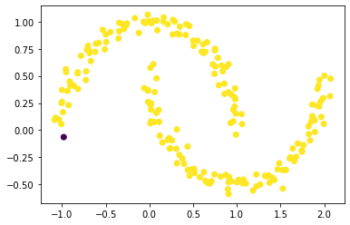
Whoops, it seems like something is wrong with either the minimization process or even older processes. That one lonely purple point still gives us some hope, so we’ll try altering the threshold of z_min for clustering.

plt.scatter(X[:,0], X[:,1], c = z_min < -.0015)

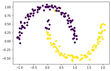
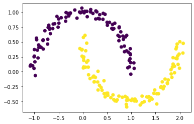
Now, the clustering seems to be working. The below plot also demonstrates that there might indeed are some issue with our optimization process.

plt.scatter(X[:,0], X[:,1], c = z < 0)

Part F: Eigen and Labels

Explicitly optimizing the orthogonal objective is way too slow to be practical. Here’s another high-light for eigenvector and eigenvalues. The significance of spectral clustering, and indeed the reason that spectral clustering is called spectral clustering, is that we can actually solve the problem from Part E using eigenvalues and eigenvectors of matrices.

Eigenvalue-eigenvector decomposition is a way of representing a matrix with more radical characteristics(basically, other matrices).

Recall that what we would like to do is minimize the function

with respect to \(\mathbf{z}\), subject to the condition \(\mathbf{z}^T\mathbf{D}\mathbb{1} = 0\).

The Rayleigh-Ritz Theorem states that the minimizing \(\mathbf{z}\) is actually to find the solution with smallest eigenvalue of the generalized eigenvalue problem

which is equivalent to the standard eigenvalue problem

Thus, the optimizing process is now left to finding the eigenvector \(\mathbf{z}\) with the second-smallest eigenvalue.

Why is it specifically the second? Indeed, \(\mathbb{1}\) is actually the eigenvector with smallest eigenvalue of the matrix \(\mathbf{D}^{-1}(\mathbf{D} - \mathbf{A})\), which is the identity matrix. So, the vector \(\mathbf{z}\) that we want must be the eigenvector with the second-smallest eigenvalue.

To find the eigenvector \(z\) with the second-smallest eigenvalue, we first construct the matrix \(\mathbf{L} = \mathbf{D}^{-1}(\mathbf{D} - \mathbf{A})\), which is often called the Laplacian matrix of the similarity matrix \(\mathbf{A}\). Then, with the handy eig function from numpy, we obtain an array of eigenvalues as Lam, and their corresponding eigen values as a matrix form, stored in U.

L = np.linalg.inv(D)@(D-A) 
Lam, U = np.linalg.eig(L)

The argsort function sorts an array and return the index array in order. We use this function to find the second-smallest eigen value, and extracts the corresponding eigen vector from U.

ix = Lam.argsort()

Lam, U = Lam[ix], U[:,ix]#reform LAM and U in sorted manner

#Lam[1], U[:,1]
z_eig = U[:,1]#extract the eigenvector z with the *second*-smallest eigenvalue

Now, we plot out the clustering result by using eigenvector \(z\) and observe how it goes

plt.scatter(X[:,0], X[:,1], c = z_eig < 0)

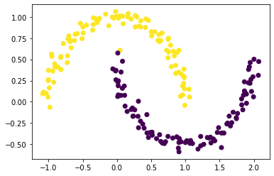
Great!

Part G: Combination: Spectral Clustering

So far, we’ve demonstrated how bi-normcut objective is calculated, how normcut is used in creating clustering labels, optimizing the labels, and how eigenvalue and vectors could be used for clustering. We’re finally ready to synthesize our work into an overall function spectral_clustering that clusters data points base off from some eigen calculation.

def spectral_clustering(X, epsilon):
    '''
    conducts spectral clustering to a set of data points 
    based on the eigenvector of the second-smallest eigenvalue of the Laplacian matrix.
    
    parameter X: a 2d n*2 array with n data points to be clustered, 
                with each entry storing the Euclidean coordinates of that point
    parameter epsilon: the threshold within which two points would be considered into one cluster
    
    return: a numpy array of size n, with entry of 1 indicating one cluster, entry of 0 indicating another,
            the nth entry corresponds to the nth data-points in the supplied X array.
    '''
    A = pairwise_distances(X)
    A = np.where(A<=epsilon, 1.0, 0.0) #set close pairs of i,js as 1s in the similarity matrix, 0 otherwise
    np.fill_diagonal(A , 0) 
    
    #compute laplacian matrix
    L = np.linalg.inv(np.diag(np.sum(A,axis=1)))@(np.diag(np.sum(A,axis=1))-A) 
    Lam, U = np.linalg.eig(L)#get the eigen value & vector of the laplacian matrix
    
    #extract the eigenvector with second-smallest eigenvalue of the Laplacian matrix
    ix = Lam.argsort()
    Lam, U = Lam[ix], U[:,ix]
    z_eig = U[:,1]
    
    return np.where(z_eig<0, 1 ,0)#returns a binary label as indicated by the eigenvector
                           

We now try out our function:

plt.scatter(X[:,0], X[:,1], c = spectral_clustering(X, epsilon))

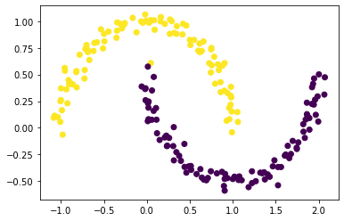
Fantastic!

Part H: exploratory of clustering ability

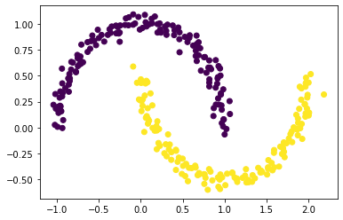
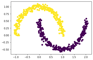
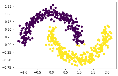
Now we’ll run a few more experiments with the spectral_clustering function. We’ll observe how varying the sample size and the noise value would influence the function’s clustering performance.

X, y = datasets.make_moons(n_samples=300, shuffle=True, noise=0.05, random_state=None)
plt.scatter(X[:,0], X[:,1], c = spectral_clustering(X, epsilon))

X, y = datasets.make_moons(n_samples=600, shuffle=True, noise=0.05, random_state=None)
plt.scatter(X[:,0], X[:,1], c = spectral_clustering(X, epsilon))

X, y = datasets.make_moons(n_samples=600, shuffle=True, noise=0.1, random_state=None)
plt.scatter(X[:,0], X[:,1], c = spectral_clustering(X, epsilon))

X, y = datasets.make_moons(n_samples=600, shuffle=True, noise=0.15, random_state=None)
plt.scatter(X[:,0], X[:,1], c = spectral_clustering(X, epsilon))

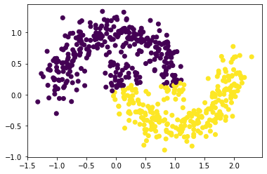
While only the sample size increases, spectral_clustering maintains its ability. However, when the noise increases, spectral_clustering shows tiredness in doing its job. This is because increasing sample size won’t affect how precise the two groups are internally, only increasing the noise would influence how the data points are spreaded, and spreadiness would involve more contact with the other cluster.

Part I: Bull’s eye demonstration

Now, we’ll try spectral_clustering on another data set – the bull’s eye!

n = 1000
X, y = datasets.make_circles(n_samples=n, shuffle=True, noise=0.05, random_state=None, factor = 0.4)
plt.scatter(X[:,0], X[:,1])

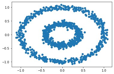
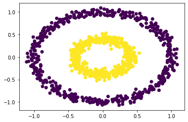
There are two concentric circles. As before k-means can’t handle this.

km = KMeans(n_clusters = 2)
km.fit(X)
plt.scatter(X[:,0], X[:,1], c = km.predict(X))

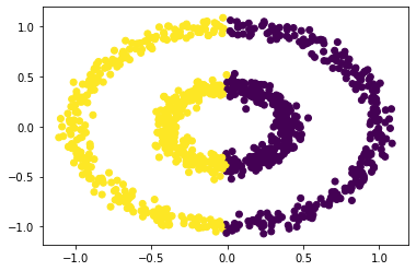
Let’s see if our spectral_clustering works!

plt.scatter(X[:,0], X[:,1], c = spectral_clustering(X, 0.4))

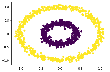
It works! Let’s sound it on its boundary of threshold.

plt.scatter(X[:,0], X[:,1], c = spectral_clustering(X, 0.5))

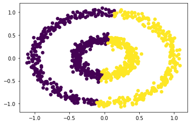
plt.scatter(X[:,0], X[:,1], c = spectral_clustering(X, 0.6))

plt.scatter(X[:,0], X[:,1], c = spectral_clustering(X, 0.7))

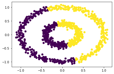
It seem like a threshold of 0.5 as the epsilon should be maintained for the spectral_clustering function to segregate the bull’s eye. Indeed reasonable, since larger epsilon would confuse the model of the intragroup closiness threshold.

=）